HMM

概述

马尔科夫链，并不是一个完美的模型。 很明显，前后关系的缺失，带来了信息的缺失:比如我们的股市，如果只是观测市场，我们只能知道当天的价格、成交量等信息， 但是并不知道当前股市处于什么样的状态(牛市、熊市、震荡、反弹等等)， 在这种情况下我们有两个状态集合，一个可以观察到的状态集合 (股市价格成交量状态等)和一个隐藏的状态集合(股市状况)。(隐藏状态是马尔科夫链，前后关系通过观测状态来补全？)

我们希望能找到一个算法可以根据股市价格成交量状况和马尔科夫假设来预测股市的状况。 在上面的这些情况下，可以观察到的状态序列和隐藏的状态序列是概率相关的。 于是我们可以将这种类型的过程建模为有一个隐藏的马尔科夫过程和 一个与这个隐藏马尔科夫过程概率相关的并且可以观察到的状态集合，就是隐马尔可夫模型。

隐马尔可夫模型(Hidden Markov Model) 是一种统计模型，用来描述一个含有隐含未知参数的马尔可夫 过程。 其难点是从可观察的参数中确定该过程的隐含参数，然后利用这些参数来作进一步的分析。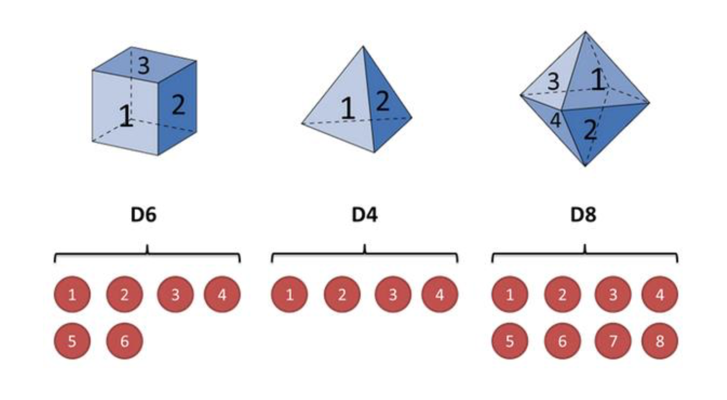

隐马尔可夫模型示意图: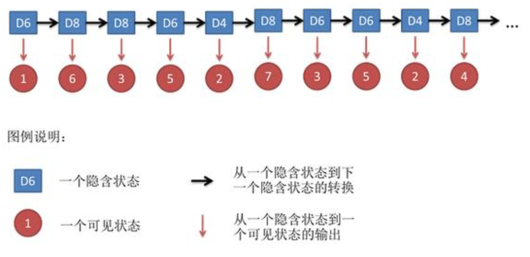

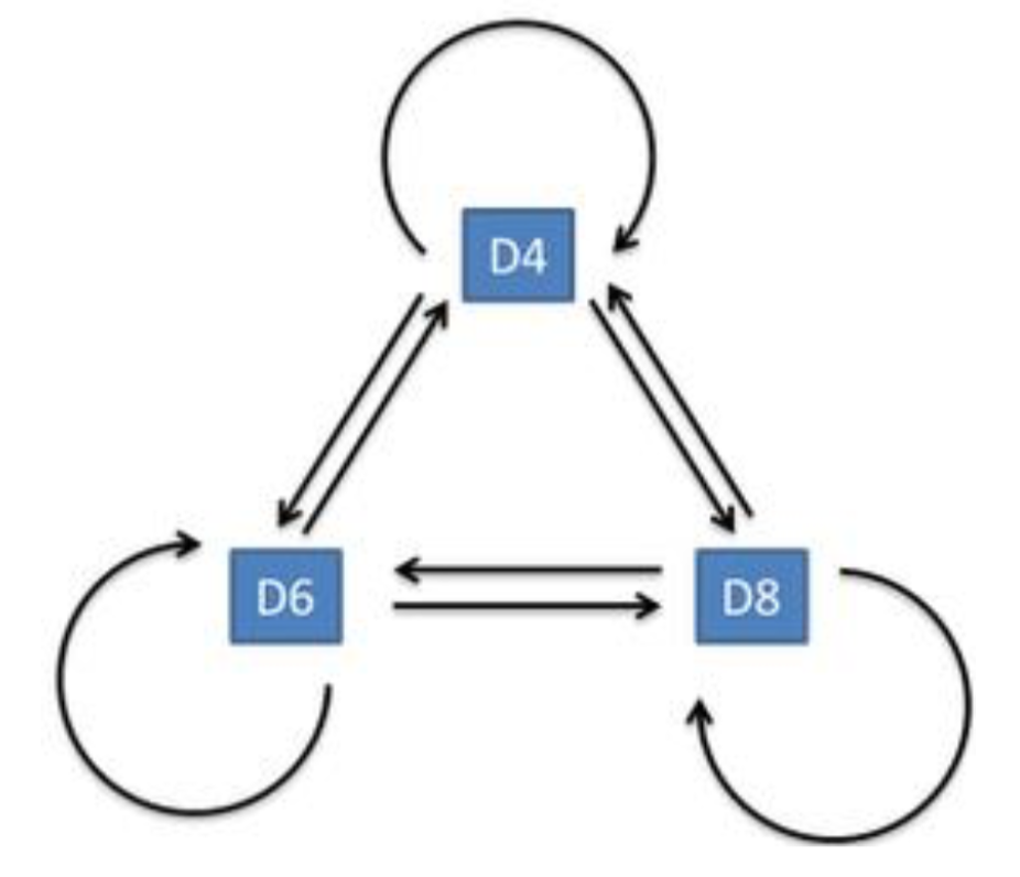
隐含状态转换示意图:

隐马尔科夫链三大问题:
1.还是知道骰子有几种(隐含状态数量)，每种骰子是什么(转换概率)， 根据掷骰子掷出的结果(可见状态链)，我想知道掷出这个结果的概率。
2.知道骰子有几种(隐含状态数量)，每种骰子是什么(转换概率)，根据掷骰子掷出的结果(可见状态链)，我想知道每次掷出来的都是哪种骰子(隐含状态链）
3.知道骰子有几种(隐含状态数量)，不知道每种骰子是什么(转换概率)， 观测到很多次掷骰子的结果(可见状态链)，我想反推出每种骰子是什么(转换概率)。
公式描述如下：
Evaluation
Given the observation sequence $O=O_{1}O_{2}…O_{T}$ and a model $\lambda = (A,B,\pi )$,how do we efficiently compute $P(O|\lambda)$, i.e., the probability of the observation sequence given the model.

Recognition
Given the observation sequence $O=O_{1}O_{2}…O_{T}$ and a model $\lambda = (A,B,\pi )$,how do we choose a corresponding state sequence $Q = q_{1}q_{2}…q_{T}$ which is optimal in some sense, i.e., best explians ths observations.

Training
Given the observation sequence $O=O_{1}O_{2}…O_{T}$, how di we adjust the model parameters $\lambda = (A,B,\pi )$ to maximize $P(O|\lambda)$.

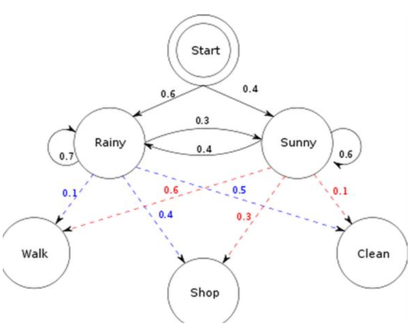
如上，初始概率分布 π；状态转移矩阵 A；观测量的概率分布 B； 同时有两个状态； 三种可能的观测值。
问题1，已知整个模型，我观测到连续三天做的事情是:散步，购物，收拾。 那么，根据模型，计算产生这些行为的概率是多少。
问题2，同样知晓这个模型，同样是这三件事，我想猜，这三天的天气是怎么样的。
问题3，最复杂的，我只知道这三天做了这三件事儿，而其他什么信息都没有。 我得建立一个模型，晴雨转换概率，第一天天气情况的概率分布， 根据天气情况选择做某事的概率分布。

解法

• 问题一： 遍历算法，前向算法（Forward Algorithm），或者后向算法（Backward Algorithm）。
• 问题二： 维特比算法（Viterbi Algorithm）。
• 问题三： 鲍姆-韦尔奇算法（Baum-Welch Algorithm）。

遍历算法

• We need $P(O|\lambda)$, i.e., the probability of the observation sequence $O=O_{1}O_{2}…O_{T}$ given the model $\lambda$.
• So we can enumerate every possible state sequence $Q = q_{1}q_{2}…q_{T}$.
• For a sample sequence Q $$P(O|Q,\lambda) = \prod_{t=1}^{T}{P(O_{t}|q_{t},\lambda)} = \prod_{t=1}^{T}{b_{q_{t}O_{t}}}$$
• The probability of such a state sequence Q is $$P(Q|\lambda) = P(q_{1})\prod_{t=2}^{T}{P(q_{t}|q_{t-1})} = \pi_{q_{1}}\prod_{t=2}^{T}{a_{q_{t-1} q_{t}}}$$
• Therefore the joint probability $$P(O,Q|\lambda) = P(Q|\lambda)P(O|Q,\lambda) = \pi_{q_{1}}\prod_{t=2}^{T}{a_{q_{t-1} q_{t}}} \prod_{t=1}^{T}{b_{q_{t}O_{t}}}$$
• By considering all possible state sequences $$P(O|\lambda) = \sum_{Q}{\pi_{q_{1}}b_{q_{1}O_{1}}\prod_{t=2}^{T}{a_{q_{t-1} q_{t}}b_{q_{t}O_{t}}}}$$
• Problem: order of $2TN^{T}$ calculations
  • $N^{T}$ possible state sequence
  • about 2T calculations for each sequence

举例其中一种隐状态序列为：雨-雨-雨

$$P(O|\lambda) = P(雨1，雨2，雨3) = P(雨1)*P(W)*P(雨2|雨1)*P(S)*P(雨3|雨2，雨1)*P(C) \\ = 0.6*0.1*0.7*0.4*0.7*0.5 = 0.00588$$

再把$N^{t}$中可能的隐状态序列累加起来：

$$P(O|\lambda) = \sum_{Q}{\pi_{q_{1}}b_{q_{1}O_{1}}\prod_{t=2}^{T}{a_{q_{t-1} q_{t}}b_{q_{t}O_{t}}}}$$

前向算法

• We define a forward variable $\alpha_{j}(t)$ as the probability of the partial observation seq. until time $t$, with state $S_{j}$ at time $t$（前向变量） $$\alpha_{j}(t) = P(O_{1}O_{2}...O_{t},q_{t}=S_{j}|\lambda)$$
• This can be computed inductively $$\alpha_{j}(1) = \pi_{j}b_{jO_{1}}, 1\leq j \leq N$$ $$\alpha_{j}(t+1) = (\sum_{i=1}^{N}{\alpha_{i}(t)a_{ij}})b_{jO_{t+1}}, 1\leq t \leq T-1$$
• Then with $N^{2}T$ operations: $$P(O|\lambda) = \sum_{i=1}^{N}{P(O,q_{T}=S_{i}|\lambda)} = \sum_{i=1}^{N}{\alpha_{i}(T)}$$ 举例，t=1 ($\alpha_{j}(1) = $)： $$P(雨1，W) = \pi_{j}b_{jO_{1}} = 0.6*0.1 = 0.06 \\ P(晴1，W) = \pi_{j}b_{jO_{1}} = 0.4*0.6 = 0.24$$ t=2($\alpha_{j}(t+1)$): $$P(雨2，S) = (\sum_{i=1}^{N}{\alpha_{i}(t)a_{ij}})b_{jO_{t+1}} \\ = (P(雨1，W)*P(雨2|雨1)+P(晴1，W)*P(雨2|晴1))*P(S|雨2) \\ = (0.06*0.7+0.24*0.4)*0.4 = 0.0552$$ $$P(晴2，S) = (\sum_{i=1}^{N}{\alpha_{i}(t)a_{ij}})b_{jO_{t+1}} \\ = (P(雨1，W)*P(晴2|雨1)+P(晴1，W)*P(晴2|晴1))*P(S|晴2)$$ 如此往下计算，t=…T;在最后把第T步的所有隐状态可能加起来即可。

（从上面的这些算法可见，马尔科夫链都是应用在隐状态上）

后向算法

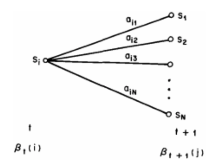
Figure:Operations for computing the backward variable $\beta_{i}(t)$ (后向变量)

• We define a backward variable $\beta_{i}(t)$ as the probability of the partial observation seq. after time $t$, given stat $S_{i}$ at time $t$. $$\beta_{i}(t) = P(O_{t+1}P_{t+2}...O_{T}|q_{t}=S_{i},\lambda)$$
• This can be computed inductively as well $$\beta_{i}(T) = 1 , 1\leq i \leq N$$ $$\beta_{i}(t-1) = \sum_{j=1}^{N}{a_{ij}b_{jO_{t}}\beta_{j}(t)} , 2\leq t \leq T$$ 举例，初始化，时刻t=3: $$\beta_{雨}(3) = 1 \\ \beta_{晴}(3) = 1$$ 时刻t=2： $$\beta_{雨}(2) = \sum_{j=1}^{N}{a_{ij}b_{jO_{t}}\beta_{j}(t)}\\ =P(雨3|雨2)*P(C|雨3)*\beta_{雨}(3)+P(晴3|雨2)*P(C|晴3)*\beta_{晴}(3)\\ = 0.7*0.5*1 + 0.3*0.1*1 = 0.38$$ $$\beta_{晴}(2) = \sum_{j=1}^{N}{a_{ij}b_{jO_{t}}\beta_{j}(t)}\\ =P(雨3|晴2)*P(C|雨3)*\beta_{雨}(3)+P(晴3|晴2)*P(C|晴3)*\beta_{晴}(3)\\ = 0.3*0.5*1 + 0.6*0.1*1 = 0.21$$ 同理计算t=1： $$\beta_{雨}(1) \beta_{晴}(1)$$ 最终计算$\beta(0)$： $$P(O|\lambda) = P(W,S,C) = \pi_{雨}*P(W|雨1)*\beta_{雨}(1) + \pi_{晴}*P(W|晴1)*\beta_{晴}(1)$$

Viterbi算法

• Finding the best single sequence means computing $argmax_{Q} P(Q|O,\lambda)$, equivalent to $argmax_{Q} P(Q,O|\lambda)$
• The Viterbi algorithm (dynamix programming) defines \delta_{j}(t), i.e., the highest probability of a single path of length $t$ which accounts for the observations and ends in state $S_{j}$ $$\delta_{j}(t) = max_{q_1,q_2,...,q_{t-1}} P(q_{1}q_{2}...q_{t}=j,O_{1}O_{2}...O_{t}|\lambda)$$
• By induction $$\delta_{j}(1) = \pi_{j}b_{jO_{1}}, 1 \leq j \leq N\\ \delta_{j}(t+1) = (max_{i}\delta_{i}(t)a_{ij})b_{jO_{t+1}}, 1\ leq t \leq T-1$$
• With backtracking (keeping the maximizing argument for each $t$ and $j$) we fing the optimal solution.

举例，t=1：

$$\delta_{雨}(1) = \pi_{雨}*P(W|雨1) = 0.6*0.1 = 0.06\\ \delta_{晴}(1) = \pi_{晴}*P(W|晴1) = 0.4*0.6 = 0.24$$

初始化路径：

$$\phi_{雨}(1) = 0\\ \phi_{晴}(1) = 0$$

t=2：

$$\delta_{雨}(2) = max[\delta_{雨}(1)*a_{雨1->雨2}|\delta_{晴}(1)*a_{晴1->雨2}]*b_{雨O_{2}}\\ =max[0.06*0.7|0.24*0.4]*0.4 = 0.096*0.4 = 0.0384\\$$

因为通过计算，由晴1->雨2概率比较大，记录最优路径$\phi_{雨}(2)$ = 晴。

$$\delta_{晴}(2) = max[\delta_{雨}(1)*a_{雨1->晴2}|\delta_{晴}(1)*a_{晴1->晴2}]*b_{晴O_{2}}\\ =max[0.06*0.3|0.24*0.6]*0.3 = 0.144*0.3 = 0.0434$$

由晴1->晴2概率比较大，记录最优路径$\phi_{晴}(2)$ = 晴。

同理，计算t=3：
记录最优路径，假设$\phi_{雨}(3)$ = 晴，$\phi_{晴}(3)$ = 雨。又假设我们计算得到$\delta_{雨}(3) \geq \delta_{晴}(3) $，所以由最后往前回溯得到路径：$\phi_{雨}(3)=晴 -> \phi_{晴}(2)=晴 -> \phi_{晴}(1) = 0$ , 即路径为：雨-晴-晴-0。

Baum-Welch算法

• There is no knoew way to analytically solve for the model which maximizes the probability of the observation sequence
• We can choose $\lambda=(A,B,\pi)$ which locally maxizizes P(O|\lambda)
  • gradient techniques (梯度下降法)
  • Baum-Welch reestimation(equivalent to EM)
• We need to define $\xi_{ij}(t)$, i.e., the probability of being in state $S_{i}$ at time $t$ and in state $S_{j}$ at time $t+1$ $$\xi_(ij) = P(q_{t}=S_{i},q_{t+1}=S_{j}|O,\lambda)$$ $$\xi_(ij) = \frac{\alpha_{i}(t)a_{ij}b_{jO_{t+1}}\beta_{j}(t+1)}{P(O|\lambda)}\\ =\frac{\alpha_{i}(t)a_{ij}b_{jO_{t+1}}\beta_{j}(t+1)}{\sum_{i=1}^{N}\sum_{i=1}^{N}\alpha_{i}(t)a_{ij}b_{jO_{t+1}}\beta_{j}(t+1)}$$ Figure: Operations for computing the $\xi_{ij}(t)$
  
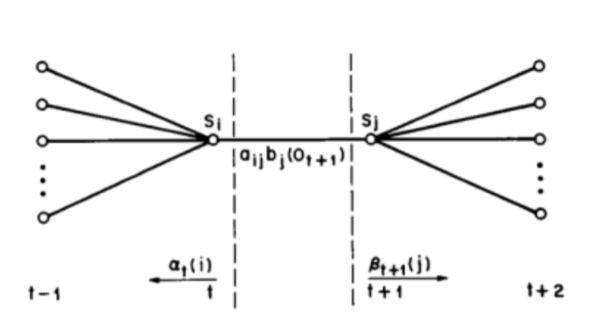
• Recall that $\gamma_{i}(t)$ is a probability of state $S_{i}$ at time $t$, hence $$\gamma_{i}(t) = \sum_{j=1}^{N}{\xi_{ij}(t)}$$
• Now if we sum over the time index t
  • $\sum_{t=1}^{T-1}{\gamma_{i}(t)}$ = expected number of times that $S_{i}$ is visited = expected number of transitions from state $S_{i}$
  • $\sum_{t=1}^{T-1}{\xi_{i}(t)}$ = expected number of transitions from $S_{i}$ to $S_{j}$
• Reestimation formulas $$\bar{\pi_{i}} = \gamma_{i}(1) \\ \bar(a_{ij}) = \frac{\sum_{t=1}^{T-1}{\xi_{i}(t)}}{\sum_{t=1}^{T-1}{\gamma_{i}(t)}} \\ \bar{b_{jk}} = \frac{\sum_{O_{t}=V_{k}}{\gamma_{j}(t)}}{\sum_{t=1}^{T}{\gamma_{j}(t)}}$$ (这里主要思想就是评率的概率，分母为总次数，分子为某一类次数)
• Baum et al. proved that if current model id $\lambda = (A,B,\pi)$ and we use the above to compute $\bar{\lambda} = (\bar{A},\bar{B},\bar{\pi})$ then either
  • $\bar{\lambda} = \lambda$ we are in a critical point if the likelihood function
  • $P(O|\bar{\lambda}) > P(O|\lambda)$ model $\bar{\lambda}$ is more likely
• If we iteratively reestimate the parameters we obtain a maximum likelihood estimate of the HMM
• Unfortunately this finds a local maximum and the surface can be very complex.
  定义出模型参数$\bar{\lambda} = (\bar{A},\bar{B},\bar{\pi})$后，就是EM算法的求解了。